GUIDE’ing Simulink with MATLAB

Introduction

Some of us Simulink users may find ourselves needing a graphical user interface (GUI) to run and interact with our dynamic simulation. For instance, we may need to modify block parameters or visualise results during the simulation, and not afterwards. Fortunately, you can.

Although Simulink does provide a programmable interface that you can call from MATLAB, this capability is rarely put into use (in fact, it is hardly even known by most users.) This article describes some of the ways in which you can utilise Simulink’s interface in MATLAB GUI.

Getting (Your Model) Started

If you look under Simulink > Functions in the Help Browser, you’ll notice that there is a huge list of functions available. You won’t be needing most of them, but knowing a few of these functions comes in handy at times.

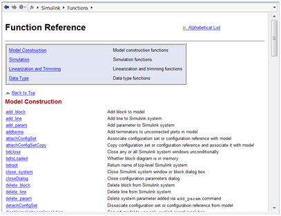
Figure 1: List of Simulink Functions in Help Browser

Below are some of the functions that I use from time to time:

open_system(‘sys’)	Opens Simulink model
close_system(‘sys’)	Closes Simulink model
paramValue = get_param(object, paramName)	Gets properties of Simulink model or the blocks
set_param(object, paramName, Value)	Sets properties of Simulink model or the blocks
bdclose(‘sys’)	Closes Simulink model unconditionally

As you can see, most of these functions are self-explanatory, and you may read about these functions from the help browser if you need more information on them. (The people at MathWorks have done a wonderful job putting up the help content, and I must admit that it’s quite a reliable answer source for most of my questions. Hence, we should all make good use of it.)

There are two functions that I would like to elaborate further: the get_param function and the set_param function. As you can tell, they are just two sides of the same coin. One allows you to get information from your model, and the other allows you to modify your model (assuming your model is already open.)

get_param

The get_param(object, paramName) function allows you to acquire information from your model. For example; if you want to check if you’re model is already running, you can type the following:

>> get_param(‘TestModel’,‘SimulationStatus’)

ans =

stopped

Likewise, the argument object also allows you to refer to the blocks within your model. For example; if you want to know the value of a manual switch (which changes between value of 1 and 0):

>> get_param(‘TestModel/Manual Switch’,‘sw’)

ans =

0

set_param

The set_param(object, paramName, Value)function allows you to modify parameters in your model. For example; you can change the simulation status with the following commands:

set_param(‘TestModel’,‘SimulationCommand’,‘start’)

set_param(‘TestModel’,‘SimulationCommand’,‘pause’)

set_param(‘TestModel’,‘SimulationCommand’,‘stop’)

Once again, it should be obvious what these commands will perform. The same can be done to Simulink blocks; you can change the block properties such as the sampling time, gain values, threshold, etc.

With this, you can easily interact with your model without touching your Simulink window, but through the command prompt or a script instead.

(Note: One of the common pitfalls with set_param and get_param is that when users have to work with numerical data, they tend to treat the parameter values as numerical data type, and this is incorrect. Simulink parameters should be treated as string types, and this applies to all numerical parameters such as ‘value’, ‘sampling time’, ‘frequency’, etc.)

Callback Functions

That should cover for most of us Simulink users. But sometimes we need more than just operating Simulink from MATLAB; can we call MATLAB functions from our Simulink environment? This could be useful, for instance, if we need to perform data analysis every time we finish running or when we pause our simulation. Another example would be when we want to load different parameter configurations for our model, and we have saved these configurations in different MAT-files.

We can automate these tasks using callback functions. There are two places where you can add callback functions: File>Model Properties if we want to specify callback functions for our model, or if we want to specify callback functions for some of the blocks, we can do so by going to the block properties.

Figure 2: Callback functions at Model Properties

Figure 3 Callback functions at Block Properties

As you can see, there are many different callback functions that you can introduce into your model. To use them, you just have to select on the desired callback function, and add in the MATLAB code that you would want to be executed. For instance, if I want to create a block that loads one of my models when I double-click on it, I can add in the following line in my OpenFcn callback:

open_system(‘myTestModel’)

If you want to know which callback to use, you may search for “Common Block Parameters” in the Help Browser and you should see the list of callback functions and the kind of situations that triggers their execution. I won’t delve into further details here, as I have seen some good articles floating around the web. Here is the link to a page which shows you how some of the more common callback functions can be put to use: http://www.mathworks.com/support/tech-notes/1800/1818.html

As for the others: Google is your friend. =)

Adding Event Listeners (For blocks)

You can add event listeners in your Simulink model so that when a block method executes, a MATLAB program is called to perform some task. The block events that you can register to are as follows:

‘PreDerivatives’

Before a block‘s Derivatives method executes

‘PostDerivatives’

After a block‘s Derivatives method executes

‘PreOutputs’

Before a block‘s Outputs method executes.

‘PostOutputs’

After a block‘s Outputs method executes

‘PreUpdate’

Before a block‘s Update method executes

‘PostUpdate’

After a block‘s Update method executes

One of the common use of the event listener is to interact with your MATLAB GUI in real time. For example, if you want to update your plot in sync with your simulation, you may do so with the event listener.

Below is a sample function that does the starts a Simulink model and adds the event listener that plots the output of the block ‘SineWave’:

function SampleFunction

ModelName = 'TestModel';

% Opens the Simulink model
open_system(ModelName);

% Simulink may optimise your model by integrating all your blocks. To
% prevent this, you need to disable the Block Reduction in the Optimisation
% settings.
set_param(ModelName,'BlockReduction','off');

% When the model starts, call the localAddEventListener function
set_param(ModelName,'StartFcn','localAddEventListener');

% Start the model
set_param(ModelName, 'SimulationCommand', 'start');

% Create a line handle
global ph;
ph = line([0],[0]);

% When simulation starts, Simulink will call this function in order to
% register the event listener to the block 'SineWave'. The function
% localEventListener will execute everytime after the block 'SineWave' has
% returned its output.
function eventhandle = localAddEventListener

eventhandle = add_exec_event_listener('TestModel/SineWave', ...
										'PostOutputs', @localEventListener);

% The function to be called when event is registered.
function localEventListener(block, eventdata)

disp('Event has occured!')
global ph;

% Gets the time and output value
simTime = block.CurrentTime;
simData = block.OutputPort(1).Data;

% Gets handles to the point coordinates
xData = get(ph,'XData');
yData = get(ph,'YData');

% Displaying only the latest n-points
n = 200;

if length(xData) <= n
	xData = [xData simTime];
	yData = [yData simData];
else
	xData = [xData(2:end) simTime];
	yData = [yData(2:end) simData];
end

% Update point coordinates

set(ph,...
	'XData',xData,...
	'YData',yData);

% The axes limits need to change as you scroll
samplingtime = .01;

%Sampling time of block 'SineWave'
offset = samplingtime*n;
xLim = [max(0,simTime-offset) max(offset,simTime)];
set(gca,'Xlim',xLim);
drawnow;

(Note: This is not meant to be a complete program. One thing that I did not show here is that you should also remove the listener using delete (eventhandle) when you have completed your simulation.)

Figure 4: TestModel

Figure 5: Live Update for your Plot

Gluing it together with GUIDE (Bringing it over in guide)

Knowing all of this code, you can easily build a GUI that interacts with your simulation model. The codes that I have mentioned above can be easily plugged into your GUI interface.

I do not intend to make this article a “How-to” for GUI, so you’ll have to read that out on your own. (At MATLAB’s command window, type ‘doc guide’and you should find all the details you need to get started.)

Below is a sample GUI that you can build fairly quickly:

Figure 6: Example GUI connected to Simulink

The example here is largely based on Phil Goddard’s submission: “Simulink Signal Viewing using Event Listeners and a MATLAB UI” in the MATLAB Central’s File Exchange. His example illustrates the integration of the MATLAB UI, Simulink model and a generic real time model using the event listeners. So if you want to find out more, here is the link: http://www.mathworks.com/matlabcentral/fileexchange/24294-simulink-signal-viewing-using-event-listeners-and-a-matlab-ui

“Tim Toady”: There is more than one way to do it

Like the old Perl adage, Simulink provides you a variety of options to interface with the MATLAB environment. It’s really up to you, the user, to decide for the right tool for the job. While the work you need to do is not going to be as straightforward as just plainly using Simulink, you know it’s worthwhile when you need it. 😉

End of the Article:

Article by Tan Yu Ang, Application Engineer